In a previous post I have shown how to create text-processing pipelines for machine learning in python using scikit-learn. The core of such pipelines in many cases is the vectorization of text using the tf-idf transformation. In this post I will show some ways of analysing and making sense of the result of a tf-idf. As an example I will use the same kaggle dataset, namely webpages provided and classified by StumbleUpon as either ephemeral (content that is short-lived) or evergreen (content that can be recommended long after its initial discovery).

Tf-idf

As explained in the previous post, the tf-idf vectorization of a corpus of text documents assigns each word in a document a number that is proportional to its frequency in the document and inversely proportional to the number of documents in which it occurs. Very common words, such as “a” or “the”, thereby receive heavily discounted tf-idf scores, in contrast to words that are very specific to the document in question. The result is a matrix of tf-idf scores with one row per document and as many columns as there are different words in the dataset.

How do we make sense of this resulting matrix, specifically in the context of text classification? For example, how do the most important words, as measured by their tf-idf score, relate to the class of a document? Or can we characterise the documents that a tf-idf-based classifier commonly misclassifies?

Analysing classifier performance

Let’s start by collecting some data about the performance of our classifier. We will then use this information to drill into specific groups of documents in terms of their tf-idf scores.

A typical way to assess a model’s performance is to score it using cross-validation on the training set. One may do that using scikit-learn’s built-in cross_validation.cross_val_score() function, but that only calculates the overall performance of the model on individual folds, and doesn’t hang on to other information that may be useful. A manual cross-validation may therefore be more appropriate. The following code shows a typical implementation of cross-validation in scikit-learn:

def analyze_model(model=None, folds=10):
''' Run x-validation and return scores, averaged confusion matrix, and df with false positives and negatives '''

X, y, X_test = load()
y = y.values   # to numpy
X = X.values
if not model:
    model = load_model()

# Manual x-validation to accumulate actual
cv_skf = StratifiedKFold(y, n_folds=folds, shuffle=False, random_state=42)
scores = []
conf_mat = np.zeros((2, 2))      # Binary classification
false_pos = Set()
false_neg = Set()

for train_i, val_i in cv_skf:
    X_train, X_val = X[train_i], X[val_i]
    y_train, y_val = y[train_i], y[val_i]

    print "Fitting fold..."
    model.fit(X_train, y_train)

    print "Predicting fold..."
    y_pprobs = model.predict_proba(X_val)       # Predicted probabilities
    y_plabs = np.squeeze(model.predict(X_val))  # Predicted class labels

    scores.append(roc_auc_score(y_val, y_pprobs[:, 1]))
    confusion = confusion_matrix(y_val, y_plabs)
    conf_mat += confusion

    # Collect indices of false positive and negatives
    fp_i = np.where((y_plabs==1) & (y_val==0))[0]
    fn_i = np.where((y_plabs==0) & (y_val==1))[0]
    false_pos.update(val_i[fp_i])
    false_neg.update(val_i[fn_i])

    print "Fold score: ", scores[-1]
    print "Fold CM: \n", confusion

print "\nMean score: %0.2f (+/- %0.2f)" % (np.mean(scores), np.std(scores) * 2)
conf_mat /= folds
print "Mean CM: \n", conf_mat
print "\nMean classification measures: \n"
pprint(class_report(conf_mat))
return scores, conf_mat, {'fp': sorted(false_pos), 'fn': sorted(false_neg)}

This function not only calculates the average score (e.g. accuracy, in this case area under the ROC-curve), but also calculates an averaged confusion-matrix (across the different folds) and keeps a list of the documents (or more generally samples) that have been misclassified (false positives and false negatives separately). Finally, using the averaged confusion matrix, it also calculates averaged classification measures such as accuracy, precision etc. The corresponding function class_report() is this:

def class_report(conf_mat):
    tp, fp, fn, tn = conf_mat.flatten()
    measures = {}
    measures['accuracy'] = (tp + tn) / (tp + fp + fn + tn)
    measures['specificity'] = tn / (tn + fp)        # (true negative rate)
    measures['sensitivity'] = tp / (tp + fn)        # (recall, true positive rate)
    measures['precision'] = tp / (tp + fp)
    measures['f1score'] = 2*tp / (2*tp + fp + fn)
    return measures

One may, for example, use the confusion matrix or classification report to compare models with different classifiers to see whether there are differences in the misclassified samples (if different models perform very similar in this regard there may be no need to “ensemblify” them).

Here I will use the false positives and negatives to see whether we can use their tf-idf scores to understand why they are being misclassified.

Making sense of the tf-idf matrix

Let’s assume we have a scikit-learn Pipeline that vectorizes our corpus of documents. Let X be the matrix of dimensionality (n_samples, 1) of text documents, y the vector of corresponding class labels, and ‘vec_pipe’ a Pipeline that contains an instance of scikit-learn’s TfIdfVectorizer. We produce the tf-idf matrix by transforming the text documents, and get a reference to the vectorizer itself:

Xtr = vec_pipe.fit_transform(X)
vec = vec_pipe.named_steps['vec']
features = vec.get_feature_names()

‘features’ here is a variable that holds a list of all the words in the tf-idf’s vocabulary, in the same order as the columns in the matrix. Next, we create a function that takes a single row of the tf-idf matrix (corresponding to a particular document), and return the n highest scoring words (or more generally tokens or features):

def top_tfidf_feats(row, features, top_n=25):
    ''' Get top n tfidf values in row and return them with their corresponding feature names.'''
    topn_ids = np.argsort(row)[::-1][:top_n]
    top_feats = [(features[i], row[i]) for i in topn_ids]
    df = pd.DataFrame(top_feats)
    df.columns = ['feature', 'tfidf']
    return df

Here we use argsort to produce the indices that would order the row by tf-idf value, reverse them (into descending order), and select the first top_n. We then return a pandas DataFrame with the words themselves (feature names) and their corresponding score.

The result of a tf-idf, however, is typically a sparse matrix, which doesn’t support all the usual matrix or array operations. So in order to apply the above function to inspect a particular document, we convert a single row into dense format first:

def top_feats_in_doc(Xtr, features, row_id, top_n=25):
''' Top tfidf features in specific document (matrix row) '''
row = np.squeeze(Xtr[row_id].toarray())
return top_tfidf_feats(row, features, top_n)

Using this to show the top 10 words used in the third document of our matrix, for example, which StumbleUpon has classified as ‘evergreen’, gives:

         feature     tfidf
0            flu  0.167878
1  prevent heart  0.130590
2    fruits that  0.128400
3     of vitamin  0.123592
4    cranberries  0.119959
5        the flu  0.117032
6      fight the  0.115101
7      vitamin c  0.113120
8        vitamin  0.111867
9        bananas  0.107010

This seems to be webpage about foods or supplements to prevent or fight flu symptoms. Let’s see if this topic is represented also in the overall corpus. For this, we will calculate the average tf-idf score of all words across a number of documents (in this case all documents), i.e. the average per column of a tf-idf matrix:

def top_mean_feats(Xtr, features, grp_ids=None, min_tfidf=0.1, top_n=25):
    ''' Return the top n features that on average are most important amongst documents in rows
        indentified by indices in grp_ids. '''
    if grp_ids:
        D = Xtr[grp_ids].toarray()
    else:
        D = Xtr.toarray()

    D[D < min_tfidf] = 0
    tfidf_means = np.mean(D, axis=0)
    return top_tfidf_feats(tfidf_means, features, top_n)

Here, we provide a list of row indices which pick out the particular documents we want to inspect. Providing ‘None’ indicates, somewhat counterintuitively, that we’re interested in all documents. We then calculate the mean of each column across the selected rows, which results in a single row of tf-idf values. And this row we then simply pass on to our previous function for picking out the top n words. One crucial trick here, however, is to first filter out the words with relatively low scores (smaller than the provided threshold). This is because common words, such as ‘a’ or ‘the’, while having low tf-idf scores within each document, are so frequent that when averaged over all documents they would otherwise easily dominate all other terms.

Calling this function with grp_ids=None, gives us the most important words across the whole corpus. Here are the top 15:

                   feature     tfidf
0                    funny  0.003522
1                   sports  0.003491
2                 swimsuit  0.003456
3                  fashion  0.003337
4                       si  0.002972
5                    video  0.002700
6           insidershealth  0.002472
7       sports illustrated  0.002329
8   insidershealth article  0.002294
9              si swimsuit  0.002258
10                    html  0.002216
11             illustrated  0.002208
12              allrecipes  0.002171
13                 article  0.002144
14                   humor  0.002143

There is no obvious pattern here, beyond the fact that sports, health, fashion and humour seem to characterize the majority of articles. What might be more interesting, though, is to separately consider groups of documents falling into a particular category. For example, let’s calculate the mean tf-idf scores depending on a document’s class label:

def top_feats_by_class(Xtr, y, features, min_tfidf=0.1, top_n=25):
    ''' Return a list of dfs, where each df holds top_n features and their mean tfidf value
        calculated across documents with the same class label. '''
    dfs = []
    labels = np.unique(y)
    for label in labels:
        ids = np.where(y==label)
        feats_df = top_mean_feats(Xtr, features, ids, min_tfidf=min_tfidf, top_n=top_n)
        feats_df.label = label
        dfs.append(feats_df)
    return dfs

This function uses the previously defined functions to return a list of DataFrames, one per document class, and each containing the top n features. Instead of printing them out as a table, let’s create a figure in matplotlib:

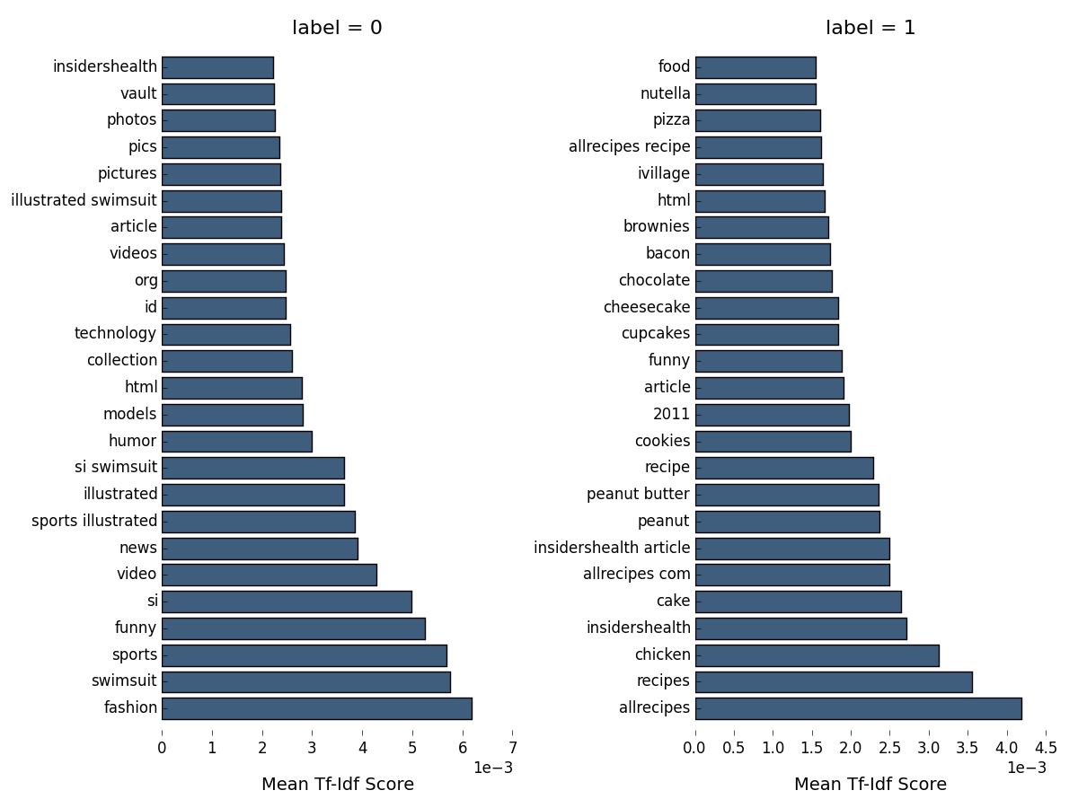
This looks much more interesting! Web pages classified as ephemeral (class label=0) seem to fall mostly into the categories of photos and videos of sports illustrated models (the abbreviation si refers to the magazine also), or otherwise articles related to fashion, humor or technology. Those pages classified as evergreen, in contrast, seem to relate mostly to health, food and recipes in particular (class label=1). This also includes, of course, the first evergreen article we identified above (about fruits and vitamins preventing flu). Some overlap also exists, however. The word ‘funny’ appears in the top 25 tf-idf tokens for both categories, as does the name of the allrecipes website. Together this tells us a little bit about the features (the presence of tokens) on the basis of which a trained classifier may categorize pages as belonging to one class or the other.

For reference, here is the function to plot the tf-idf values using matplotlib:

def plot_tfidf_classfeats_h(dfs):
    ''' Plot the data frames returned by the function plot_tfidf_classfeats(). '''
    fig = plt.figure(figsize=(12, 9), facecolor="w")
    x = np.arange(len(dfs[0]))
    for i, df in enumerate(dfs):
        ax = fig.add_subplot(1, len(dfs), i+1)
        ax.spines["top"].set_visible(False)
        ax.spines["right"].set_visible(False)
        ax.set_frame_on(False)
        ax.get_xaxis().tick_bottom()
        ax.get_yaxis().tick_left()
        ax.set_xlabel("Mean Tf-Idf Score", labelpad=16, fontsize=14)
        ax.set_title("label = " + str(df.label), fontsize=16)
        ax.ticklabel_format(axis='x', style='sci', scilimits=(-2,2))
        ax.barh(x, df.tfidf, align='center', color='#3F5D7D')
        ax.set_yticks(x)
        ax.set_ylim([-1, x[-1]+1])
        yticks = ax.set_yticklabels(df.feature)
        plt.subplots_adjust(bottom=0.09, right=0.97, left=0.15, top=0.95, wspace=0.52)
    plt.show()

As a last step, let’s plot the top tf-df features for webpages misclassified by our full text-classification pipeline, using the indices of false positive and negatives identified above:

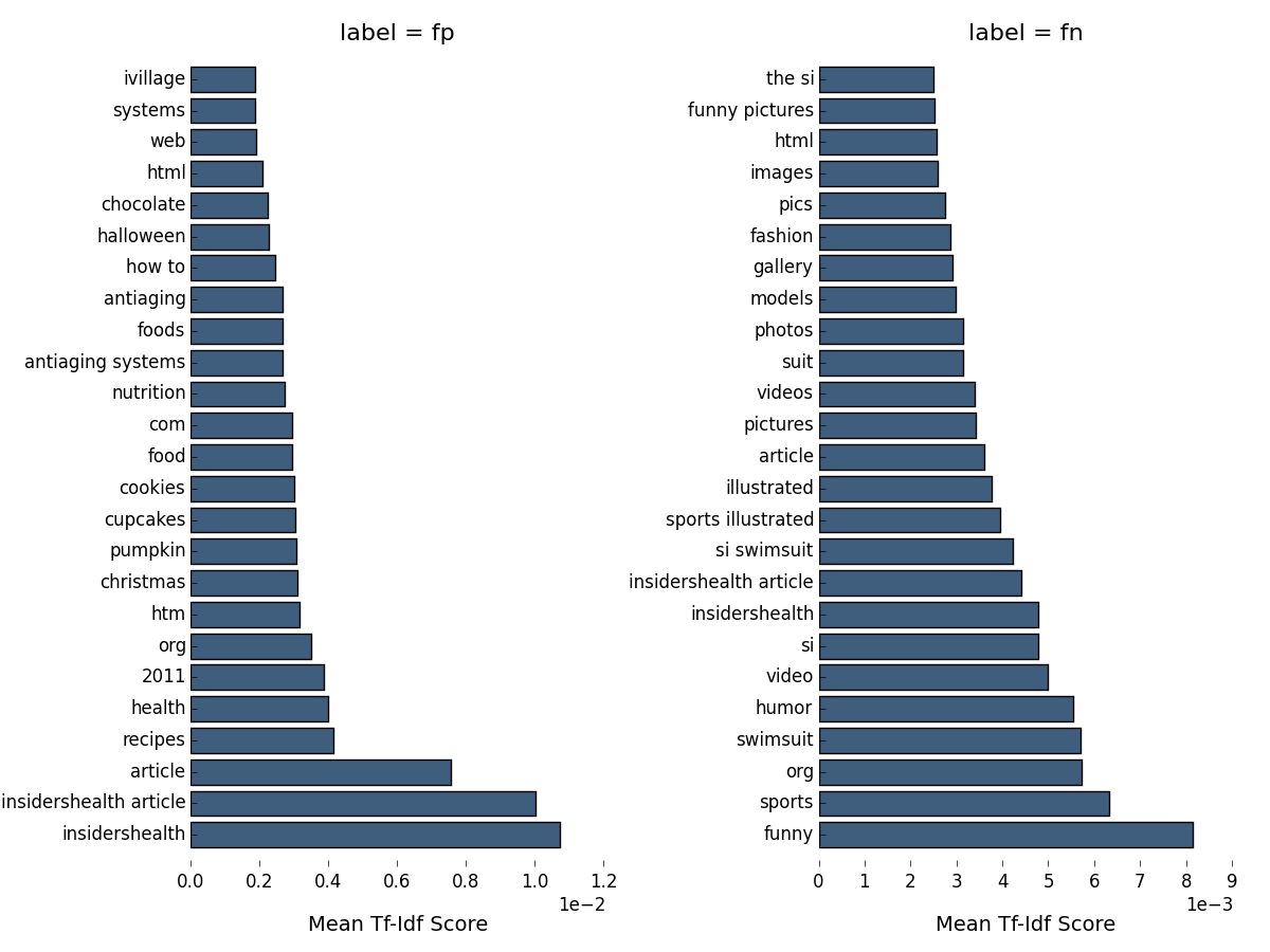
Unfortunately we can at best get some initial hints as to the reason for misclassification from this figure. Our false positives are very similar to the true positives, in that they are also mostly health, food and recipe pages. One clue may be the presence of words like christmas and halloween in these pages, which may indicate that their content is specific to a particular season or date of the year, and therefore not necessarily recommendable at other times. The picture is similar for the false negatives, though in this case there is nothing at all indicating any difference with true positives. One would probably have to dig a little deeper into individual cases here to see how they may differ.

Final thoughts

This post barely scratches the surface of how one might go about analyzing the results of a tf-idf transformation in python, and is directed primarily at people who may use it as a black box algorithm without necessarily knowing what’s inside. There may be many other, and probably better ways of going about this. I nevertheless think it’s a useful tool to have around. Note that a similar analysis of top features amongst a group of documents could be applied also after clustering the documents first. One could then use the cluster index, instead of the class label, to group documents and plot their top tf-idf tokens to get further insight about the specific characteristics of each cluster.